A better confusion matrix with python
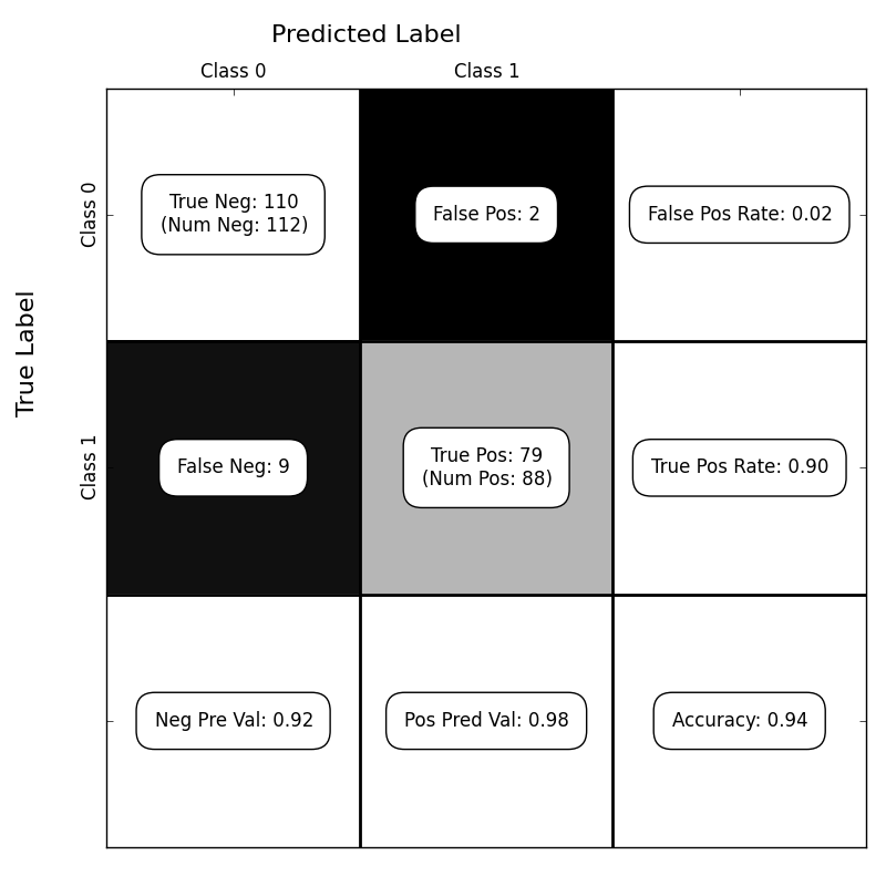
The Confusion Matrix is a nice way to summarize the results from a binary classification problem. While scikit-learn offers a nice method to compute this matrix (for multiclass classification, as well), I’m not aware of a built-in method that shows the relevant statistics from the confusion matrix. Often the matrix is just shown, color-coded according to entry values.
I wrote a little script for displaying the confusion matrix (as computed by scikit-learn), using matplotlib. The results look like this:
Here’s the function for generating the confusion matrix:
def show_confusion_matrix(C,class_labels=['0','1']):
    """
    C: ndarray, shape (2,2) as given by scikit-learn confusion_matrix function
    class_labels: list of strings, default simply labels 0 and 1.

    Draws confusion matrix with associated metrics.
    """
    import matplotlib.pyplot as plt
    import numpy as np

    assert C.shape == (2,2), "Confusion matrix should be from binary classification only."

    # true negative, false positive, etc...
    tn = C[0,0]; fp = C[0,1]; fn = C[1,0]; tp = C[1,1];

    NP = fn+tp # Num positive examples
    NN = tn+fp # Num negative examples
    N  = NP+NN

    fig = plt.figure(figsize=(8,8))
    ax  = fig.add_subplot(111)
    ax.imshow(C, interpolation='nearest', cmap=plt.cm.gray)

    # Draw the grid boxes
    ax.set_xlim(-0.5,2.5)
    ax.set_ylim(2.5,-0.5)
    ax.plot([-0.5,2.5],[0.5,0.5], '-k', lw=2)
    ax.plot([-0.5,2.5],[1.5,1.5], '-k', lw=2)
    ax.plot([0.5,0.5],[-0.5,2.5], '-k', lw=2)
    ax.plot([1.5,1.5],[-0.5,2.5], '-k', lw=2)

    # Set xlabels
    ax.set_xlabel('Predicted Label', fontsize=16)
    ax.set_xticks([0,1,2])
    ax.set_xticklabels(class_labels + [''])
    ax.xaxis.set_label_position('top')
    ax.xaxis.tick_top()
    # These coordinate might require some tinkering. Ditto for y, below.
    ax.xaxis.set_label_coords(0.34,1.06)

    # Set ylabels
    ax.set_ylabel('True Label', fontsize=16, rotation=90)
    ax.set_yticklabels(class_labels + [''],rotation=90)
    ax.set_yticks([0,1,2])
    ax.yaxis.set_label_coords(-0.09,0.65)


    # Fill in initial metrics: tp, tn, etc...
    ax.text(0,0,
            'True Neg: %d\n(Num Neg: %d)'%(tn,NN),
            va='center',
            ha='center',
            bbox=dict(fc='w',boxstyle='round,pad=1'))

    ax.text(0,1,
            'False Neg: %d'%fn,
            va='center',
            ha='center',
            bbox=dict(fc='w',boxstyle='round,pad=1'))

    ax.text(1,0,
            'False Pos: %d'%fp,
            va='center',
            ha='center',
            bbox=dict(fc='w',boxstyle='round,pad=1'))


    ax.text(1,1,
            'True Pos: %d\n(Num Pos: %d)'%(tp,NP),
            va='center',
            ha='center',
            bbox=dict(fc='w',boxstyle='round,pad=1'))

    # Fill in secondary metrics: accuracy, true pos rate, etc...
    ax.text(2,0,
            'False Pos Rate: %.2f'%(fp / (fp+tn+0.)),
            va='center',
            ha='center',
            bbox=dict(fc='w',boxstyle='round,pad=1'))

    ax.text(2,1,
            'True Pos Rate: %.2f'%(tp / (tp+fn+0.)),
            va='center',
            ha='center',
            bbox=dict(fc='w',boxstyle='round,pad=1'))

    ax.text(2,2,
            'Accuracy: %.2f'%((tp+tn+0.)/N),
            va='center',
            ha='center',
            bbox=dict(fc='w',boxstyle='round,pad=1'))

    ax.text(0,2,
            'Neg Pre Val: %.2f'%(1-fn/(fn+tn+0.)),
            va='center',
            ha='center',
            bbox=dict(fc='w',boxstyle='round,pad=1'))

    ax.text(1,2,
            'Pos Pred Val: %.2f'%(tp/(tp+fp+0.)),
            va='center',
            ha='center',
            bbox=dict(fc='w',boxstyle='round,pad=1'))


    plt.tight_layout()
    plt.show()
… and here’s the code that generates the above example:
import numpy as np
from sklearn.linear_model import LogisticRegression
from sklearn.metrics import confusion_matrix
from show_confusion_matrix import show_confusion_matrix

rs = np.random.RandomState(1234)
p = 2
n = 200
py1 = 0.6
mean1 = np.r_[1,1.]
mean0 = -mean1

# generate training data
Y = (rs.rand(n) > py1).astype(int)
X = np.zeros((n,p))
X[Y==0] = rs.multivariate_normal(mean0, np.eye(p), size=(Y==0).sum())
X[Y==1] = rs.multivariate_normal(mean1, np.eye(p), size=(Y==1).sum())

lr = LogisticRegression()
lr.fit(X,Y)

# generate test data
Y = (rs.rand(n) > py1).astype(int)
X = np.zeros((n,p))
X[Y==0] = rs.multivariate_normal(mean0, np.eye(p), size=(Y==0).sum())
X[Y==1] = rs.multivariate_normal(mean1, np.eye(p), size=(Y==1).sum())

C = confusion_matrix(Y,lr.predict(X))
show_confusion_matrix(C, ['Class 0', 'Class 1'])