The ROC curve Part 2 - Numerical Example with Python

This short post is a numerical example (with Python) of the concepts of the ROC curve and AUC score introduced in this post using the logistic regression example introduced in theory here and numerically with Python here.

First let’s import the usual libraries and set some parameters:

import numpy as np
import matplotlib.pyplot as plt

rs = np.random.RandomState(4321)
p = 2
n = 200
py1 = 0.6
mean1 = np.r_[1,1.]
mean0 = -mean1

# These are the parameters learned through maximization from before.
w = np.r_[2.45641058, 1.55227045]
b = -0.824723538369

Next, we generate testing data which will be used to generate the ROC curve and AUC score. We also compute the logistic regression model’s prediction for this testing data.

# Generate some testing data
Y = (rs.rand(n) > py1).astype(int)
X = np.zeros((n,p))
X[Y==0] = rs.multivariate_normal(mean0, np.eye(p), size=(Y==0).sum())
X[Y==1] = rs.multivariate_normal(mean1, np.eye(p), size=(Y==1).sum())

# This is the model's prediction on the test data.
T = 1 / (1. + np.exp(-b-np.dot(X,w)))

Next, we generate $TP(t), TN(t), FP(t), FN(t)$ using a discrete number of thresholds. From these we generate $FPR(t)$, $TPR(t)$, and the ROC curve.

thresholds = np.linspace(1,0,101)

ROC = np.zeros((101,2))

for i in range(101):
    t = thresholds[i]

    # Classifier / label agree and disagreements for current threshold.
    TP_t = np.logical_and( T > t, Y==1 ).sum()
    TN_t = np.logical_and( T <=t, Y==0 ).sum()
    FP_t = np.logical_and( T > t, Y==0 ).sum()
    FN_t = np.logical_and( T <=t, Y==1 ).sum()

    # Compute false positive rate for current threshold.
    FPR_t = FP_t / float(FP_t + TN_t)
    ROC[i,0] = FPR_t

    # Compute true  positive rate for current threshold.
    TPR_t = TP_t / float(TP_t + FN_t)
    ROC[i,1] = TPR_t

# Plot the ROC curve.
fig = plt.figure(figsize=(6,6))
plt.plot(ROC[:,0], ROC[:,1], lw=2)
plt.xlim(-0.1,1.1)
plt.ylim(-0.1,1.1)
plt.xlabel('$FPR(t)$')
plt.ylabel('$TPR(t)$')
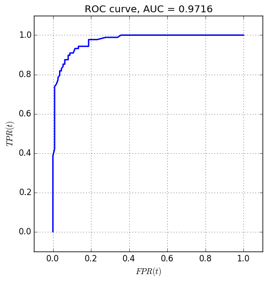
plt.grid()

Finally, we compute the AUC score for the ROC curve using the trapezoidal method, and show the plot.

AUC = 0.
for i in range(100):
    AUC += (ROC[i+1,0]-ROC[i,0]) * (ROC[i+1,1]+ROC[i,1])
AUC *= 0.5

plt.title('ROC curve, AUC = %.4f'%AUC)
plt.show()

This produces: