Machine Learning Part 2 - Numerical Example with Python
This post is a continuation of the previous introduction to binary classification. I’ll go over some Python code to implement the logistic model discussed in the previous post. We’ll use simple gradient ascent to find the model parameters.
Sample data
Consider $p=2$, $P(Y=1)=0.6$, and $P(X|Y=j) \sim \mathcal{N}(\mu_j, I)$ where $I$ is the identity matrix and $\mu_0 = \begin{bmatrix} -1 & -1 \end{bmatrix}^T$, $\mu_1 = \begin{bmatrix} 1 & 1 \end{bmatrix}^T$. We can generate some sample data with $n=200$ (realizations of the random variables $\mathbf{X}$ and $\mathbf{Y}$ mentioned in the previous post) using the following:
import numpy as np

rs = np.random.RandomState(1234)
p = 2
n = 200
py1 = 0.6
mean1 = np.r_[1,1.]
mean0 = -mean1

Y = (rs.rand(n) > py1).astype(int)
X = np.zeros((n,p))
X[Y==0] = rs.multivariate_normal(mean0, np.eye(p), size=(Y==0).sum())
X[Y==1] = rs.multivariate_normal(mean1, np.eye(p), size=(Y==1).sum())
…and we can plot the data with:
import matplotlib.pyplot as plt
plt.plot(X[Y==0,0], X[Y==0,1], 'ob', label='Class 0')
plt.plot(X[Y==1,0], X[Y==1,1], 'sr', label='Class 1')
plt.legend(loc=2, numpoints=1)

plt.show()
which generates:
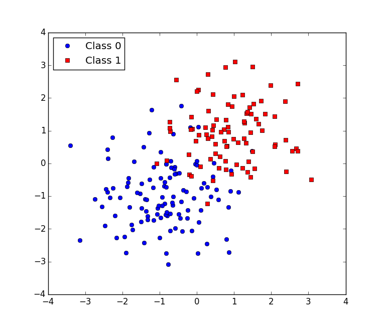
Visually, we can see the data should be able to be separated by a line fairly well.
Partial derivatives
We assume the parameters are independent. We assume $b$ is uniform with a large range (no regularization), and $w$ are gaussian with variance $1/\lambda$. So,
\[\begin{align*} D_bl(w,b) &= \sum_{i=1}^n y^i - g(x^i|w,b) =: \sum_{i=1}^n (Y-G)_i \\ D_{w_k}l(w,b) &= -\lambda w_k + \sum_{i=1} (y^i - g(x^i|w,b))x_k^i \\ D_wl(w,b) &= -\lambda w + X^T(Y-G) \end{align*}\]The definitions of the vectors, $G$ and $Y$, allow us to compute the gradient with respect to all of $w$ more efficiently using the matrix-vector product. Note that $\lambda$ is a free regularization parameter to be set. Finally, we take gradient ascent steps from some initial parameters using a fixed step size, $\eta$:
\[\begin{align*} b &\leftarrow b + \eta \cdot D_bl(w,b) \\ w &\leftarrow w + \eta \cdot D_wl(w,b) \end{align*}\]Let’s implement this:
def gradient_ascent(w, b, lamb, eta, n_iters):
    # G is P(Y=1|X) under the current parameters.
    G = 1 / (1. + np.exp(-b-np.dot(X,w)))
    # loss is the function we're maximizing
    loss = -lamb * np.log(w**2).sum() + np.log(G[Y==1]).sum() + np.log(1-G[Y==0]).sum()
    print "iteration:", 0, "| loss:", loss, "| accuracy:", ((G>0.5) == Y).mean()

    for iter in range(1, n_iters+1):
        G = 1 / (1. + np.exp(-b-np.dot(X,w)))
        loss = -lamb * 0.5 * (w**2).sum() + np.log(G[Y==1]).sum() + np.log(1-G[Y==0]).sum()
        print "iteration:", iter, "| loss:", loss, "| accuracy:", ((G>0.5) == Y).mean()

        # Now, do gradient ascent.
        ymg    = Y-G
        grad_b = ymg.sum()
        grad_w = -lamb * w + np.dot(ymg,X)

        b += eta*grad_b
        w += eta*grad_w
    return w,b
and write a little test suite:
init_w = rs.randn(X.shape[1])
init_b = rs.rand()*50-25

w,b=gradient_ascent(w=init_w.copy(), b=init_b, lamb=0., eta=0.01, n_iters=10)

print "\n"

print "Parameters found ... w:", w, "b:", b

# Generate some new testing data
Y_ = (rs.rand(n) > py1).astype(int)
X_ = np.zeros((n,p))
X_[Y_==0] = rs.multivariate_normal(mean0, np.eye(p), size=(Y_==0).sum())
X_[Y_==1] = rs.multivariate_normal(mean1, np.eye(p), size=(Y_==1).sum())

G = 1 / (1. + np.exp(-b-np.dot(X_,w)))

print "\n"

print "Accuracy on test data:", ((G>0.5) == Y_).mean()
This outputs:
iteration: 0 | loss: -296.149573246 | accuracy: 0.555
iteration: 1 | loss: -296.149573246 | accuracy: 0.555
iteration: 2 | loss: -146.967673727 | accuracy: 0.68
iteration: 3 | loss: -91.5016877875 | accuracy: 0.79
iteration: 4 | loss: -70.761997325 | accuracy: 0.84
iteration: 5 | loss: -60.5078209358 | accuracy: 0.875
iteration: 6 | loss: -54.6336803289 | accuracy: 0.89
iteration: 7 | loss: -50.9696103327 | accuracy: 0.89
iteration: 8 | loss: -48.5475798159 | accuracy: 0.9
iteration: 9 | loss: -46.877202585 | accuracy: 0.9
iteration: 10 | loss: -45.6881194776 | accuracy: 0.905


Parameters found ... w: [ 2.45641058  1.55227045] b: -0.824723538369


Accuracy on test data: 0.93
It is very important to test the model on a data set held out from the parameter learning process. Although it is fine to monitor the progress of the learning process using the data set used for learning parameters, scores for the model should not be reported using this data unless it is made completely explicit. It is the scores on data not used to learn parameters that provide insight as to how the model might generalize to unseen data. Thus, these scores are more truthful to report.
Note that I ignored the regularization term. It turns out to be not significant for this toy problem (try it yourself). However, in problems where $n$ is small, $p$ is large, or both, regularization can help tremendously.
Finally let’s visualize the predictions made over the region and the decision boundary:
x,y = np.mgrid[-4:4:61j,-4:4:61j]
xy = np.c_[ x.flatten(), y.flatten() ]

G = 1 / (1. + np.exp(-b-np.dot(xy,w)))

fig = plt.figure()
# This is a color coding of the numerical prediction over the region.
plt.contourf(x, y, G.reshape(x.shape), cmap=plt.cm.bwr, alpha=0.6)

x1 = (-b-4*w[1]) / w[0]
x2 = (-b+4*w[1]) / w[0]
# This draws the decision boundary.
plt.plot( [x1,x2], [4, -4.], '-k', lw=3)

plt.plot(X[Y==0,0], X[Y==0,1], 'ob')
plt.plot(X[Y==1,0], X[Y==1,1], 'sr')

plt.show()
This produces:
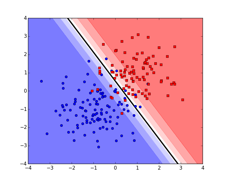
And that’s all. You can download all the above scripts in one file here.