Decision boundary preserving PCA
Suppose we train a linear classifier on some data, and we’d like to project the data onto a few dimensions for visualization in such a way that respects the boundary of the classifier in some optimal way. This means we should project the data parallel to the hyperplane defining the decision surface in a way that minimizes the distance between the point in the original space and the projection.
For convenience, let’s suppose that the hyperplane passes through the origin. We can always subtract off the intercept to make this true anyway. In this case, the separating hyperplane is defined by the unit vector, $w \in \mathbb{R}^p$. Suppose $X \in \mathbb{R}^{n \times p}$ is the matrix of training examples, $x_i \in \mathbb{R}^p$, used to create the classifier.
Let’s suppose, we want to project the data onto two dimensions. One of these directions should be $w$. The other direction, say $u$, should be orthogonal to $w$, and we can also require it to be unit length. We want to minimize the average squared error when projecting the data onto $w$ and $u$. That is, we want to solve:
\[\min_u \sum_{i=1}^n ||(ww^T + uu^T)x_i - x_i||^2 \;\; \text{subject to} \;\; u^Tu=1, \; w^Tu = 0\]If you set up the Lagrangian, differentiate, and all that, you arrive at the following necessary condition:
\[Su = (w^TSu)w + (u^TSu)u\]where $S = X^TX$
Intuitively, we are choosing the best plane to project the data, subject to the constraint that plane is orthogonal to the vector that defines the decision boundary, and thus projects parallel to the decision boundary (hyperplane).
The above looks like an eigenvalue problem. Let’s consider an augmented eigenvalue problem for the scatter matrix, $S$. Suppose $Q \in \mathbb{R}^{p \times p-1}$ spans the space orthogonal to $w$, i.e., $Q^Tw = 0 \in \mathbb{R}^{p-1}$. The project of the data onto $Q$ is $XQQ^T$. If we perform standard PCA on the projected data, we must solve:
\[QQ^TX^TX QQ^T u = \lambda u\]or
\[QQ^TSQQ^T u = \lambda u\]It is immediate that $w$ is the only eigenvector with null eigenvalue since the matrix on the left is rank $p-1$. If $u$ is an eigenvector with non-null eigenvalue, then it follows from the above that $w^Tu = 0$. We can also force $u^Tu = 1$. Furthmore, note that since $P = [w \; Q]$ is full rank with orthonormal columns, then $PP^T = ww^T + QQ^T = I \in \mathbb{R}^{p \times p}$.
So if $u$ is an eigenvector to the augmented scatter matrix eigenvalue problem above,
\[\lambda = u^TQQ^TSQQ^Tu = u^T(ww^T + QQ^T)S(ww^T+QQ^T)u = u^TSu\]so that:
\[\begin{align*} Su &= (ww^T+QQ^T)Su \\ &= (w^TSu)w + QQ^TSu \\ &= (w^TSu)w + QQ^TS(ww^T + QQ^T)u \\ &= (w^TSu)w + QQ^TSQQ^Tu \\ &= (w^TSu)w + (u^TSu) u \\ \end{align*}\]Thus if $u$ is a solution to the “projection eigenvalue equation”, it is a solution to the above minimization problem. One can verify that we should take the eigenvector associate with the greatest eigenvalue.
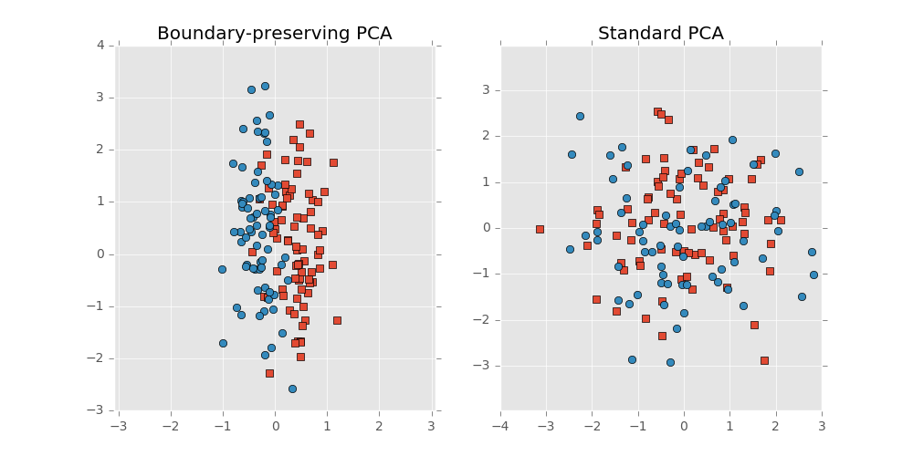
Let’s consider an example comparing the decision boundary preserving method to standard PCA where the the two classes are separated by a noisy hyperplane and the data is distributed with lesser variance in the direction normal to the hyperplane. So the data looks like an $p$ dimensional disk, or coin, with the two classes residing on either face of the coin. Standard PCA, not knowing anything of the class structure or decision boundary, squashes the classes onto one another. The above method projects the data onto a subspace in the direction of the thin edge of the disk since this direction is parallel to the decision boundary.
Here’s a visualization: