What is the ROC curve?!

The ROC curve as well as the area under the curve (AUC) score are frequently used in binary classification to characterize the quality of an automatic classifier. In this post, I define the ROC curve and AUC score as theoretical probabilistic quantities and use these definitions to show important properties. Next, I derive empirical estimates from the theoretical definitions using a finite sample and show that these estimates coincide with what are given as the “usual” definitions of the sensitivity, specificity, and the ROC curve.

This post builds on a previous introductory post on the binary classification problem, so you should be familiar with the notation and terminology there if you don’t want this to sound like gibberish. Although, if you have a familiarity with machine learning and pattern recognition, the notation and terminology used here should be familiar as well.

Preliminaries

Recall that our discriminative model, $g(x|\theta) = P(Y=1|X=x,\theta)$, has fixed parameters learned through a maximization process. Let $T = g(X|\theta)$ be the random quantity which is the output of the classifier. Hence, the range of $T$ is $[0,1]$. Previously, we implicitly assumed that a label of $1$ is assigned when $T \gt 0.5$ and label $0$ is assigned when $T \leq 0.5$. The goal of ROC analysis is to observe threshold values other than $0.5$ in order to make trade-offs between true and false positivity.

To be clear, this whole analysis could be done assuming the range of $T$ is any subset or possibly all of $\mathbb{R}$. I assume the range above so that this post is cohesive with my previous post on binary classification. What’s really important is that $T$ is to be interpreted as some scalar value for which we must apply a threshold to say it belongs to one of two classes. Afterwards, our decision based on this threshold may or may not agree the ground truth label, $Y$.

Events of label and classifier agreement

Recall that we assumed we had a sample $\{(X^i, Y^i)\}_{i=1}^n$ where each pair, $(X^i, Y^i)$, is identically distributed and also independent of every other pair, $(X^j, Y^j)$, for $i \neq j$. With this being the case, we say that the tuples, $(X^i, Y^i)$, are iid. It follows that the tuples, $(T^i, Y^i)$, are also iid. I frequently drop the sample index when referring to a single observation or when speaking of the distributions of these quantities.

We’re interested in the joint distribution of $(T,Y)$ so that we can examine quantities like $P(T \gt t, Y=1)$, i.e. the probability of a true positive event for a threshold value of $t$. There are other events that we’re interested in. For example, $P(T \leq t, Y=1)$ is the probability of a false negative event. There are two other joint events, namely true negative and false positive events defined in the obvious way.

We can make the following empirical estimate:

$\mathbb{I}$ is the indicator function who is $1$ if the argument is true and $0$ otherwise. So, $\text{TP}(t)$ is the empirical number of true positive examples using a threshold of $t$ for the given sample. Similar estimates can be made for the probability of a true negative, false negative, and false positive:

These estimates are valid asymptotically due to the iid assumption and the Glivenko–Cantelli theorem.

Now, for example, using these estimates, we can measure empirical accuracy:

However, accuracy alone isn’t always the best measure of success. Measures of “false positivity” and “false negativity” are also important to consider in many situations.

Conditional classifier predictions

We just saw that accuracy essentially measures the probability of co-occurrence of agreement between the classifier and label. A similar but different question to ask pertains to the classifiers prediction conditioned on the label taking a particular value. So for instance, we might be interested in the probability that the classifier takes a value above the threshold, $t$, given that the label is $1$. For the ROC curve in particular, we’re interested in $P(T \gt t | Y=1)$ and $P(T \gt t | Y=0)$. Before we estimate these probabilities, we need to discuss an important subtlety:

In the previous section we were able to estimate the probabilities of the joint distributions because the tuples $(T^i, Y^i)$ are assumed to be iid. Since $(T^i,Y^i)$ are iid, it makes sense to talk about $P(T,Y)$ generally since $P(X^1, Y^1) = \cdots = P(X^n, Y^n)$. This is the identically distributed part of iid. So, when I wrote $P(T|Y)$ previously, it doesn’t have any meaning unless when know the conditional distribution is the same, i.e. $P(T^1|Y^1=y^i) = \cdots = P(T^n|Y^n=y^n)$. Thus, the question is: are $T^i|Y^i=y^i$ iid given that $(T^i, Y^i)$ are iid? It turns out (and is easily verified) that this is true if and only if we make the additional assumption that the $Y^i$ are iid. So, let’s assume this.

Now back to business, the conditional distributions are easy to estimate by applying Bayes’ rule and using the previous estimates of the joint distributions:

$\text{TPR}(t)$ and $\text{FPR}(t)$ stand for the empirical true positive rate and false positive rate (at threshold level $t$), respectively. $\text{TPR}(t)$ also goes by sensitivity, hit-rate, or recall. It approximates the probability of the event that the classifier will predict $1$ given that the true label is $1$. $\text{FPR}(t)$ is also known as the fall-out or $1$-specificity. It approximates the probability that the classifier will predict label $1$ given that the true label is $0$. Again, these empirical estimates coincide with the usual definitions.

The ROC curve

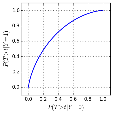
We define the ROC curve as the following parametric curve:

Each component is the complementary cumulative distribution function (complementary CDF) of $T$ conditioned on a label type. Here is an example ROC curve where $T|Y=1$ and $T|Y=0$ both follow a Beta distribution:

Plotting the ROC curve allows us to visualize how the true positive rate changes as a function of the false positive rate for various threshold values. It allows us to find a threshold which makes a compromise between the two.

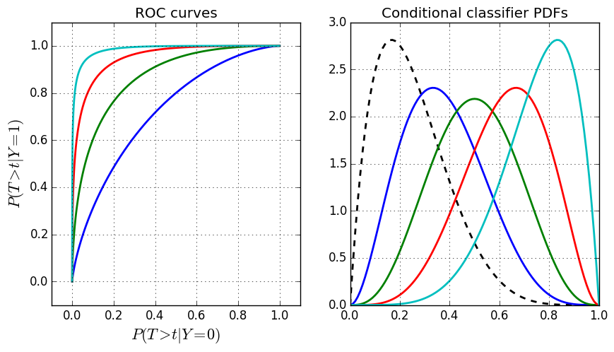
In the above figure, I’ve plotted the ROC curves on the left together with the underlying probability density functions (PDFs) on the right (still Beta distributions). Remember that the ROC curve is composed of the complementary cumulative distribution functions. The black dotted PDF on the right is the distribution of $T|Y=0$. The colored distributions are $T|Y=1$ for different Beta distribution parameters. These colors correspond to the ROC curves in the left figure with the distribution of $T|Y=0$ remaining the same in each curve. Notice the behavior of the ROC curves as the corresponding PDFs become more separated.

Let’s examine some properties of the ROC curve so that we can explain this behavior.

Properties of the ROC curve

1. $r(0) = (1,1)$
2. $r(1) = (0,0)$
3. $r(t)$ is non-increasing in each component.

So when $t$ goes from $0$ to $1$, the ROC curve starts from the point $(1,1)$, ends at $(0,0)$, and is confined to the unit square, $[0,1]^2$. It is just a matter of annoyance that the curve goes right to left as $t$ goes from $0$ to $1$. We could just as easily take $t$ from $1$ to $0$. The important thing is to remember that $t$ represents a threshold — the dividing line between class $0$ and class $1$. Property 3 says the curve doesn’t loop back on itself.

The worst curve

Consider the following:

So a straight line from $(0,0)$ to $(1,1)$ is the worst possible ROC curve. It means the classifier’s prediction is independent of the label, which is no better than a classifier that guesses randomly. Remember that independence intuitvely means the outcome of one random variable gives us no information about the outcome of another. Ideally, observing $T$ would tell us a lot about $Y$.

The best curve

Consider a curve which travels along the top then down the left side of the unit cube, i.e. straight from $(1,1)$ to $(0,1)$, and then straight from $(0,1)$ to $(0,0)$. This being the case, there must exist some threshold existing in correspondence with the top-left corner — call it $t^*$ — such that $P(T \gt t^* | Y=1) = 1$ and $P(T \gt t^* | Y=0) = 0$. From this, it follows that:

and similarly, $P(T \leq t^*) = P(Y=0)$. Clearly, this is most we could ask for from the classifier. If the distributions of $T|Y=0$ and $T|Y=1$ have densities, this case essentially means that the densities have non-intersecting support, and this value $t^*$ is placed such that the density of $T|Y=1$ lies strictly above and the density of $T|Y=0$ lies strictly below.

It is interesting to note that the opposite curve — i.e. one that travels along the right side and bottom of the unit cube — yields the opposite conclusion as above. In this case, the classifier predicts perfectly wrong.

Empirical estimate of the ROC curve

Given a discretization of $m$ threshold values, $1 = t_1 \gt t_2 \gt \cdots \gt t_{m} = 0$, we can form the empirical ROC curve as an interpolation between the points, $\{ (FPR(t_j), TPR(t_j)), \; j=1,\ldots,m \}$. Usually, a simple piecewise linear interpolation is used. By defining the threshold values this way, the points go from left to right, which is useful when computing the corresponding area underneath these points.

AUC score

The AUC score summarizes the ROC curve to a single scalar value by summing the area underneath the ROC curve. For a parametric curve, $z(t) = [x(t), \; y(t)]^T$, recall that the area underneath is given by $\int y(t) x’(t) dt$. We assume for simplicity from here on out that $T|Y=y$, $y=0,1$ admit density functions so that $P’(T \gt t|Y=y) = -p(t|Y=y)$. Recalling properties 1 & 2 of the ROC curve above, we integrate from $t=1$ to $t=0$ to obtain a positive area:

Note that an AUC score of $1$ is still only possible in the best curve case. However, while the worst ROC curve yields an AUC score of $0.5$, the converse is not necessarily true. Take, for example, an ROC curve which goes straight from $(1,1)$ to $(1,0.5)$, $(1,0.5)$ to $(0,0.5)$, and from $(0,0.5)$ to $(0,0)$. This is a valid ROC curve with AUC score of $0.5$.

Interpreting the AUC score

Let’s take two random classifier and label pairs, $(T^i, Y^i)$ and $(T^j, Y^j)$ ($i \neq j$), and ask the following question: What is the probability that the value for $T^i$ will be greater than $T^j$ given that the corresponding labels are $Y^i=1$ and $Y^j=0$?

Let’s write this out:

Aha! So the previous question is answered exactly by the AUC score. We should point out a couple of things: 1) The first step of splitting the joint distribution of $T^i, T^j | Y^i=1, Y^j=0$ requires both the iid assumption on $(T^i,Y^i)$ and $Y^i$, and 2) the indices are dropped in the last step again due to the iid assumptions.

Empirical estimate of the AUC score

Finally, the estimate of the ROC curve is just an interpolation between points in the plane, and so the AUC is easy to estimate using various numerical methods. For example, if piecewise linear interpolation is used to approximate the ROC curve, the trapezoidal rule yields:

In a separate post, I give a numerical example of the estimation of the ROC and AUC.

References