What is PCA?!
Principle component analysis or PCA is a widely-used method for dimensionality reduction. In this post, I will derive the method from a least squares error perspective using linear algebra. Therefore, I do not specifically plan to motivate its use (although I hope to aid your intuition through the derivation).
Preliminaries
You have $n$ data samples, $\mathbf{x}_1, \ldots, \mathbf{x}_n$, where $\mathbf{x}_i \in \mathbb{R}^p$. I assume that these observations have been normalized to have zero mean. We can stack these into a matrix:
\[X = \begin{bmatrix} \mathbf{x}_1^T \\ \mathbf{x}_2^T \\ \vdots \\ \mathbf{x}_n^T \\ \end{bmatrix}\]Note that $X \in \mathbb{R}^{n \times p}$. I’d like to point out that:
\[X^TX = \sum_j \mathbf{x}_j\mathbf{x}_j^T =: S \in \mathbb{R}^{p \times p}\]This is sometimes called the “scatter matrix”. If we divide it by $n$, it is the maximum likelihood estimate of the covariance matrix assuming the $\mathbf{x}_j$ are zero mean i.i.d. multivariate gaussian. I will assume that $\text{rank}(S) = p$, which is reasonable for $n \gt \gt p$.
The best 1D subspace for the data
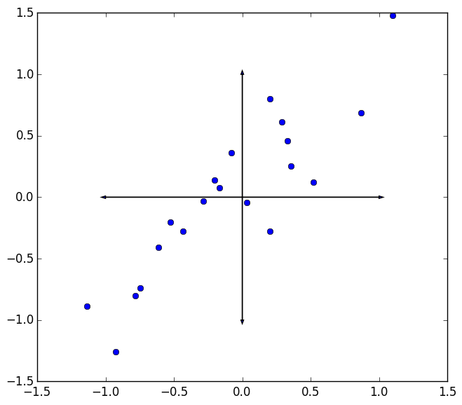
Ok then. So we have this set of data points. For the sake of visualization, we take $p=2$ as shown below. Now, here’s the question: given a point set, what is the best single direction to project all the data onto? We could project the data onto a higher dimensional subspace (some hyperplane), but for now just consider projecting all the data onto a line.
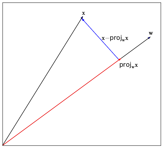
Recall that the projection of a vector, $\mathbf{x}$, onto the vector $\mathbf{w}$ is given by:
\[\text{proj}_{\mathbf{w}}\mathbf{x} = \frac{\mathbf{w}\mathbf{w}^T}{\mathbf{w}^T\mathbf{w}}\mathbf{x}\]so that the squared error incurred from projecting $\mathbf{x}$ onto $\mathbf{w}$ is
\[\text{squared error} = ||\mathbf{x} - \frac{\mathbf{w}\mathbf{w}^T}{\mathbf{w}^T\mathbf{w}}\mathbf{x}||^2\]This is illustrated in the figure below.
Thus, we seek a single direction, $\mathbf{w}$, which minimizes:
\[\begin{align*} f(\mathbf{w}) &= \sum_{i=1}^n ||\mathbf{x}_i - \frac{\mathbf{w}\mathbf{w}^T}{\mathbf{w}^T\mathbf{w}}\mathbf{x}_i||^2 \\ &= \sum_i \mathbf{x}_i^T\mathbf{x}_i - \frac{(\mathbf{x}_i^T\mathbf{w})^2}{\mathbf{w}^T\mathbf{w}} \end{align*}\]Writing the second term a little differently reveals something interesting:
\[f(\mathbf{w}) = \sum_i \mathbf{x}_i^T\mathbf{x}_i - \sum_i \frac{\mathbf{w}^T\mathbf{x}_i\mathbf{x}_i^T\mathbf{w}}{\mathbf{w}^T\mathbf{w}}\]or bringing the sum inside the second term…
\[f(\mathbf{w}) = \sum_i \mathbf{x}_i^T\mathbf{x}_i - \frac{\mathbf{w}^TS\mathbf{w}}{\mathbf{w}^T\mathbf{w}}\]You might recognize the second term as the Rayleigh quotient for eigvenvalues of $S$. Thus to minimize this function, we should set $\mathbf{w}$ to be the eigenvector of $S$ corresponding the largest eigenvalue of $S$.
Error from projecting onto a 1D space
If we call the eigenvector / eigenvalue pair $\mathbf{w}_1$ / $\lambda_1$, the error from projecting all the data onto $\mathbf{w}_1$ is:
\[\sum_i \mathbf{x}_i^T\mathbf{x}_i - \lambda_1\]However, notice that:
\[\sum_i \mathbf{x}_i^T\mathbf{x}_i = \text{trace}(XX^T) = \text{trace}(X^TX) = \text{trace}(S) = \sum_j \lambda_j\]So sum of squared errors is:
\[\sum_{j=2}^{p} \lambda_j\]This is an absolute error measure. We could make it a relative error by measuring:
\[\frac{ \sum_{j=2}^{p} \lambda_j } { \sum_{j=1}^{p} \lambda_j }\]The quantity,
\[1 - \frac{ \sum_{j=2}^{p} \lambda_j } { \sum_{j=1}^{p} \lambda_j } = \frac{\lambda_1}{\sum_{j=1}^{p} \lambda_j}\]is sometimes referred to as the “variance retained”. This would be the “variance retained” by projecting the data onto a single line. We can “preserve more variance” or reduce the sum of squared errors further by projecting onto more dimensions as I explain below.
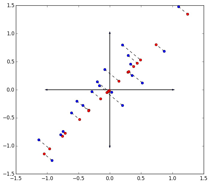
The errors are visualized below as the sum of squared distances from the original data in blue to their projection on the first eigenvector of the scatter matrix in red.
Projecting onto higher dimensions
Of course, we rarely are fortunate enough to be able to project reduce our data to a subspace of a single dimension, meaning the sum of squared errors is usually unacceptably high (variance retained too small) when projecting everything onto a single line. Usually, we project onto the first $k$ of $p$ eigenvectors of $S$.
The relative squared error for projecting the first $k$ eigenvectors of $S$ is then:
\[\frac{ \sum_{j=k+1}^{p} \lambda_j } { \sum_{j=1}^{p} \lambda_j }\]The derivation for projecting onto higher dimensions follows analogous to the previous case. I derive it here for completeness, but there’s not really more going on except for a few required tricks.
Let $W_k \in \mathbb{R}^{p \times k}$ denote the subspace of dimension $k$ that we project our data onto, minimizing the sum of squares error. That is, we seek to minimize:
\[\begin{align*} f(W_k) &= \sum_i ||\mathbf{x}_i - W_k(W_k^TW_k)^{-1}W_k^T\mathbf{x}_i||^2 \\ &= \sum_i \mathbf{x}_i^T\mathbf{x}_i - \mathbf{x}_i^TW_k(W_k^TW_k)^{-1}W_k^T\mathbf{x}_i \end{align*}\]Let’s look at the second term, and drop the subscript $k$ for clarity. We want to maximize this term to minimize the whole quantity. Let’s pull a trick, writing this scalar as the trace of a $1 \times 1$ matrix, to use the cyclic property of the trace.
\[\begin{align*} \sum_i \mathbf{x}_i^TW(W^TW)^{-1}W^T\mathbf{x}_i &= \sum_i \text{trace}(\mathbf{x}_i^TW(W^TW)^{-1}W^T\mathbf{x}_i) \\ &= \sum_i \text{trace}(\mathbf{x}_i\mathbf{x}_i^TW(W^TW)^{-1}W^T) \\ &= \text{trace}(\sum_i \mathbf{x}_i\mathbf{x}_i^TW(W^TW)^{-1}W^T) \\ &= \text{trace}(S W(W^TW)^{-1}W^T) \\ &= \text{trace}((W^TW)^{-1}W^TSW) \\ &=: \text{trace}(B) \\ &= \sum_{j=1}^k \mu_j \end{align*}\]We use the linearity of the trace, and denote the eigenvalues of the $k \times k$ matrix $B$ as $\mu_j$. So, we want to set $W$ so as to maximize the eigenvalues of this matrix $B$ which we’ve defined above. Let’s write out the eigenvector / eigenvalue equation for $B$:
\[\begin{align*} B\mathbf{u}_j &= \mu_j \mathbf{u}_j \\ (W^TW)^{-1}W^TSW\mathbf{u}_j &= \mu_j \mathbf{u}_j \\ W^TSW\mathbf{u}_j &= \mu_j W^TW\mathbf{u}_j \\ \frac{\mathbf{u}_j^TW^TSW\mathbf{u}_j}{\mathbf{u}_j^TW^TW\mathbf{u}_j} &= \mu_j \\ \end{align*}\]Let $\mathbf{y}_j = W\mathbf{u}_j$. This says that
\[\mu_j = \frac{\mathbf{y}_j^TS\mathbf{y}_j}{\mathbf{y}_j^T\mathbf{y}_j}\]So again, we have the eigenvalues of the scatter matrix, $S$ — only now, we have $k$ options. Since we want the maximum sum, we choose the first $k$ eigenvectors corresponding to the largest $k$ eigenvalues to stack into $W$. Since $S$ is real and symmetric, its eigenvectors are orthogonal. Thus the projection $\mathbf{x}_i$ onto the space is
\[W_k^T\mathbf{x}_i\]I’ll note in passing that these eigenvectors are found computationally by computed the singular value decomposition $X=USV^T$. The right singular vectors, $V$, are the eigenvectors of $S = X^TX$.